Getting Started
We demonstrate how to generate a network with scola.
An example data, sample.txt, is available on GitHub, which is composed of L=300 rows and N=25 columns (space separated), where L is the number of samples and N is the number of variables (i.e., nodes). The following code loads the data.
import numpy as np
import pandas as pd

X = pd.read_csv("https://raw.githubusercontent.com/skojaku/scola/master/data/sample.txt", header=None, sep=" ").values
L = X.shape[0] # Number of samples
N = X.shape[1] # Number of nodes
Then, compute the sample correlation matrix by
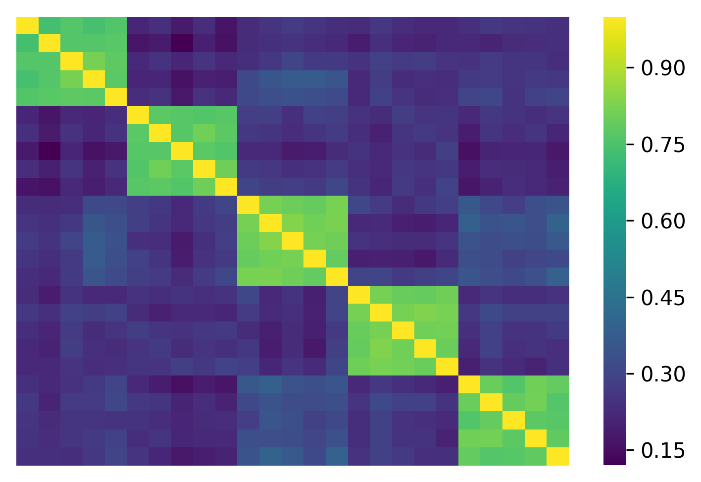
C_samp = np.corrcoef(X.T) # NxN correlation matrix
C_samp looks like
Finally, provide C_samp and L to estimate the network and associated null model:
import scola
W, C_null, selected_null_model, EBIC, construct_from, all_networks = scola.corr2net.transform(C_samp, L)
W is the weighted adjacency matrix of the generated network, where
W[i,j] indicates the weight of the edge between nodes i and j.
The W looks like
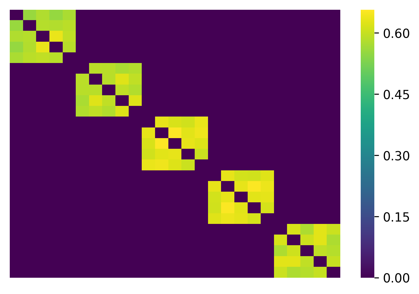
See the scola package for other return values.
Scola can construct a network from precision matrices, which is often different from that constructed from correlation matrices.
To do this, give an extra parameter construct_from='pres':
import scola
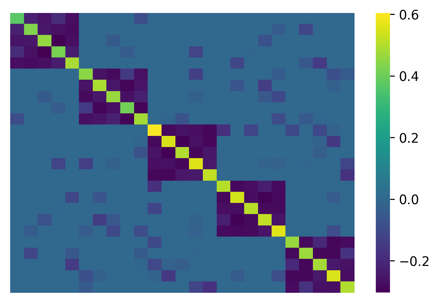
W, C_null, selected_null_model, EBIC, construct_from, all_networks = scola.corr2net.transform(C_samp, L, construct_from="pres")
which produces a different network:
If one sets construct_from='auto', the Scola constructs networks from correlation matrices and precision matrices.
Then, it chooses the one that best represents the given data in terms of the extended BIC.
The selected type of the matrix is indicated by construct_from in the return variables.